ABINIT DDB phonons
Unfold phonons from an ABINIT DDB (derivatives database) onto a
primitive cell: the route runs ABINIT’s anaddb through abipy to
obtain the supercell eigenvectors along your path, then computes the
unfolding weights with gauge-robust Bloch-sum projectors and
degenerate-group resolution, so eigenvector storage gauges do not
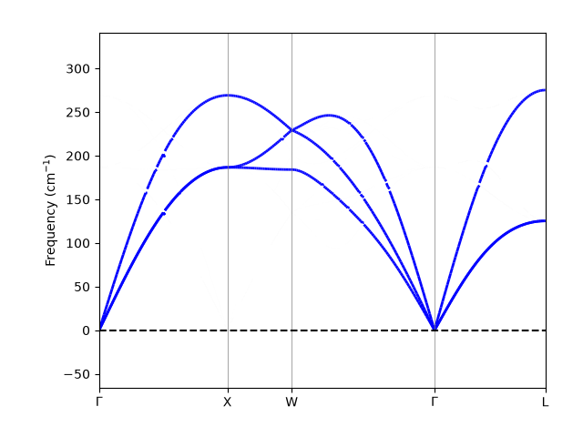
change the weights. Two bundled systems: fcc Cu from a
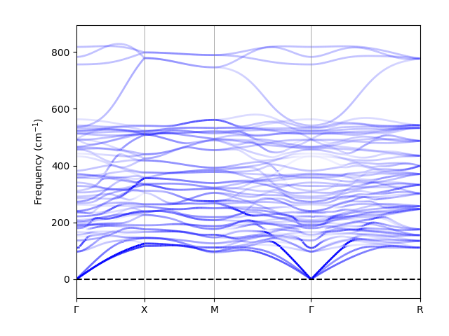
conventional-cubic-cell DDB, and CaTiO₃ from its 20-atom Pnma cell onto
the 5-atom pseudo-cubic cell.
The bundle
Download abinit-ddb.tar.gz and unpack it:
tar xf abinit-ddb.tar.gz && cd abinit-ddb
Shipped: both DDBs (data/out_DDB Cu, data/out.DDB CaTiO₃ — the
files behind the published figures), the SCF + DFPT decks that produced
them (inputs/), the pseudopotentials (pseudos/), two unfolding
configs (unfold.toml for Cu, unfold-catio3.toml), and
reproduce.py. Prerequisites: pip install "unfolding[abipy]" and a
working anaddb on your PATH (or configured in abipy’s
manager.yml).
Structure and k-path — the part that bites
Cu: the DDB stores the conventional cubic cell (natom 4) with
sc_mat = [[-1,1,1],[1,-1,1],[1,1,-1]], i.e. DDB cell = sc_mat @
primitive. Mind the k-path frame: ase’s get_special_points returns
fcc points in primitive-cell fractional coordinates, while abipy
reads path vertices in the fractional frame of the cell stored in the
DDB — for this DDB, X=(0,1,0), W=(1/2,1,0), L=(1/2,1/2,1/2). The
configs therefore pass explicit vertices in the DDB frame; anaddb
interpolates between consecutive vertices (no point density needed).
CaTiO₃: the DDB cell is the Pnma ground-state cell (20 atoms,
a ≈ b ≈ √2·a_pc, c ≈ 2·a_pc); sc_mat = [[1,-1,0],[1,1,0],[0,0,2]]
has the Pnma axes as rows in pseudo-cubic units (A_Pnma = sc_mat @
A_pc). The vertices are the pseudo-cubic Γ–X–M–Γ–R points in the DDB
frame; dipdip toggles the dipole-dipole (LO-TO) treatment passed to
anaddb (0 for CaTiO₃, as published; 1 for Cu).
Run parameters and shared options (mode, spin, method, resolve_degenerate, supercell-matrix row convention, k-path coordinates and frames, energy-reference conventions) are explained together in the method, parameters, and k-path guide.
Primitive cell input: not used by the abinit-ddb route — the path frame defaults to the cell stored in the DDB.
Configuration
# ABINIT DDB phonons: fcc Cu from a conventional-cubic-cell DDB.
# Run from the unpacked bundle root (requires anaddb on PATH, pip install unfolding[abipy]):
#   unfolding --config unfold.toml
# or with explicit flags:
#   unfolding abinit-ddb --ddb data/out_DDB \
#     --sc-mat -1 1 1 1 -1 1 1 1 -1 \
#     --kpoints 0 0 0  0 1 0  0.5 1 0  0 0 0  0.5 0.5 0.5 \
#     --names G X W G L --output cu_fcc_unfolded_cli.png
#
# The k-path vertices are the fcc special points expressed in the
# fractional frame of the cell stored in the DDB (the conventional cubic
# cell): X=(0,1,0), W=(1/2,1,0), L=(1/2,1/2,1/2). abipy interpolates
# between consecutive vertices; no point density is needed.
route = "abinit-ddb"

[input]
ddb = "data/out_DDB"                   # Cu conventional-cubic-cell DDB (natom 4)

[structure]
sc_mat = [[-1, 1, 1], [1, -1, 1], [1, 1, -1]]   # DDB cell = sc_mat @ primitive cell

[path]
kpoints = [[0, 0, 0], [0, 1, 0], [0.5, 1, 0], [0, 0, 0], [0.5, 0.5, 0.5]]
names = ["G", "X", "W", "G", "L"]

[options]
dipdip = 1                             # dipole-dipole (LO-TO) treatment

[output]
output = "cu_fcc_unfolded_cli.png"
Run it
From the unpacked bundle directory, one command per system with the shipped configs:
unfolding --config unfold.toml            # Cu     -> cu_fcc_unfolded_cli.png
unfolding --config unfold-catio3.toml     # CaTiO3 -> catio3_unfolded_cli.png
The same TOML can be passed as the only Python input:
from unfolding import load_config, run
run(load_config("unfold.toml"))         # Cu
run(load_config("unfold-catio3.toml"))  # CaTiO3
or with explicit flags (Cu):
unfolding abinit-ddb --ddb data/out_DDB \
    --sc-mat -1 1 1 1 -1 1 1 1 -1 \
    --kpoints 0 0 0 0 1 0 0.5 1 0 0 0 0 0.5 0.5 0.5 \
    --names G X W G L --output cu_fcc_unfolded_cli.png
or through the Python API with explicit parameters:
import numpy as np
from unfolding.DDB_unfolder import DDB_unfolder

# Conventional cell = sc_mat @ primitive cell
sc_mat = np.linalg.inv(np.array([[0, 1, 1], [1, 0, 1], [1, 1, 0]]) / 2.0)
knames = [r"$\Gamma$", "X", "W", r"$\Gamma$", "L"]
kpath_bounds = [[0, 0, 0], [0, 1, 0], [0.5, 1, 0], [0, 0, 0], [0.5, 0.5, 0.5]]

ax = DDB_unfolder("data/out_DDB", sc_mat=sc_mat,
                  kpath_bounds=kpath_bounds, knames=knames)
CaTiO₃ (data/out.DDB) takes the same form with
sc_mat=[[1,-1,0],[1,1,0],[0,0,2]], vertices
[[0,0,0],[0,.5,0],[.5,.5,0],[0,0,0],[.5,.5,.5]], names
Γ-X-M-Γ-R and dipdip=0. reproduce.py renders both published figures:
python reproduce.py                       # Cu     -> cu_unfolded.png
python reproduce.py --system catio3       #        -> catio3_unfolded.png
Producing your own DDB
A phonon DDB comes from an ABINIT response-function run: a
ground-state SCF, then a DFPT run with optdriver 1, rfphon 1,
rfatpol 1 natom, rfdir 1 1 1, one q-point per run (nqpt 1,
qpt 0 0 0, …), prtddb 1; merge partial DDBs with mrgddb. The
bundled inputs/ decks are worked examples for both systems.